Notes based on the book Sutton, R. S., & Barto, A. G. (2018). Reinforcement learning: An introduction. MIT press.
This chapter focuses on the evaluative aspect of reinforcement learning in a simplified, non-associative setting (one state). The core problem is balancing exploration (gathering information) and exploitation (using current information to maximize reward).
1. The -Armed Bandit Problem You are faced with (or ) different actions (levers). Each action provides a reward drawn from a probability distribution specific to that action. The goal is to maximize the expected total reward over a time period.
Greedy Action: The action with the highest estimated value. Selecting it is exploitation.
Nongreedy Action: Selecting any other action is exploration, which improves estimates of nongreedy actions.
2. Action-Value Methods We estimate the value of an action, , typically by averaging the rewards received so far for that action.
-Greedy Methods: A greedy method always exploits. An -greedy method behaves greedily most of the time but selects a random action with small probability . This ensures all actions are sampled infinitely over time.
3. Incremental Implementation To avoid storing all rewards, we update estimates incrementally using a step size. The general update rule is:
For stationary problems, the step size is (sample average).
4. Nonstationary Problems If the “true” values of actions change over time, we weight recent rewards more heavily by using a constant step-size parameter . This creates an exponential, recency-weighted average.
5. Optimistic Initial Values Initializing action-value estimates to a high value (e.g., +5 when rewards are usually < 1) encourages early exploration. The agent is “disappointed” by initial rewards and switches actions rapidly until estimates converge.
6. Upper-Confidence-Bound (UCB) Action Selection Instead of exploring randomly (like -greedy), UCB selects actions based on their potential to be optimal, considering both the estimate and the uncertainty:
The square root term represents variance/uncertainty. It decreases as an action is visited more.
7. Gradient Bandit Algorithms Instead of estimating action values, these learn numerical preferences . Action probabilities are determined via a softmax distribution. Updates are performed using stochastic gradient ascent.
Python Implementation & Visualization
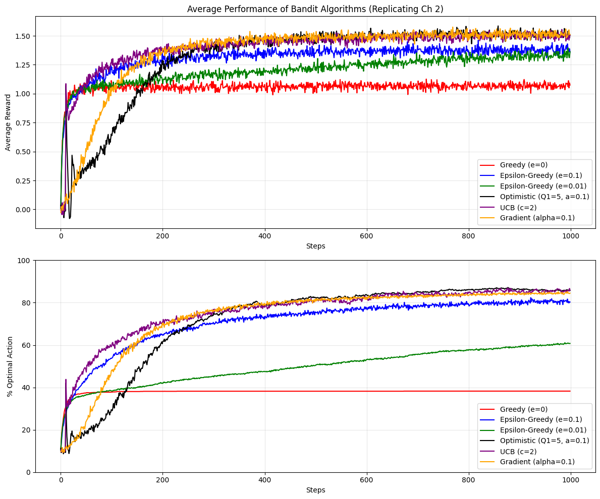
This Python code implements the 10-armed bandit testbed described in the book. It compares -Greedy, Optimistic Initialization, UCB, and Gradient Bandit algorithms.
import numpy as npimport matplotlib.pyplot as pltclass BanditProblem:def__init__(self, k=10, true_mean=0, true_variance=1):# q*(a): True values of actions (normally distributed)self.q_true = np.random.normal(true_mean, true_variance, k)# Optimal action is the index of the max true valueself.optimal_action = np.argmax(self.q_true)self.k = kdef get_reward(self, action):# Reward is selected from a normal distribution around q*(a)# Rt ~ N(q*(a), 1) return np.random.normal(self.q_true[action], 1)class Agent:def__init__(self, k=10, epsilon=0, alpha=None, initial_value=0, ucb_c=None, gradient=False, gradient_baseline=True):self.k = kself.epsilon = epsilonself.alpha = alpha # Step sizeself.ucb_c = ucb_cself.gradient = gradientself.gradient_baseline = gradient_baseline# Initializationifself.gradient:self.H = np.zeros(k) # Preferences [cite: 191]self.avg_reward =0# For baselineself.prob_actions = np.ones(k) / kelse:self.q_est = np.full(k, float(initial_value)) # Qt(a) [cite: 166]self.action_counts = np.zeros(k) # Nt(a)self.time_step =0def select_action(self):self.time_step +=1# 1. Gradient Bandit Selection [cite: 191]ifself.gradient: exp_H = np.exp(self.H - np.max(self.H)) # Stability trickself.prob_actions = exp_H / np.sum(exp_H)return np.random.choice(self.k, p=self.prob_actions)# 2. UCB Selection ifself.ucb_c isnotNone:# Add small epsilon to avoid division by zero uncertainty =self.ucb_c * np.sqrt(np.log(self.time_step) / (self.action_counts +1e-5))return np.argmax(self.q_est + uncertainty)# 3. Epsilon-Greedy Selection if np.random.rand() <self.epsilon:return np.random.randint(self.k)else:# Break ties randomly for greedy actions max_val = np.max(self.q_est) candidates = np.where(self.q_est == max_val)[0]return np.random.choice(candidates)def update(self, action, reward):# 1. Gradient Update [cite: 192]ifself.gradient:ifself.gradient_baseline:self.avg_reward += (reward -self.avg_reward) /self.time_step baseline =self.avg_rewardelse: baseline =0 one_hot = np.zeros(self.k) one_hot[action] =1# H_{t+1}(a) update# If a = At: H + alpha * (R - R_bar)(1 - pi)# If a != At: H - alpha * (R - R_bar)piself.H +=self.alpha * (reward - baseline) * (one_hot -self.prob_actions)return# 2. Action-Value Updateself.action_counts[action] +=1# Determine step size: 1/n (sample average) or constant alpha step_size =1.0/self.action_counts[action] ifself.alpha isNoneelseself.alpha# Equation 2.3 / 2.5: NewEstimate <- OldEstimate + StepSize * Error [cite: 174, 177]self.q_est[action] += step_size * (reward -self.q_est[action])# Simulation parameterssteps =1000runs =2000# Number of runs to average over (as per book figures) # Define agents to compareconfigs = [ {"label": "Greedy (e=0)", "eps": 0, "col": "red"}, {"label": "Epsilon-Greedy (e=0.1)", "eps": 0.1, "col": "blue"}, {"label": "Epsilon-Greedy (e=0.01)", "eps": 0.01, "col": "green"}, {"label": "Optimistic (Q1=5, a=0.1)", "eps": 0, "alpha": 0.1, "init": 5.0, "col": "black"}, {"label": "UCB (c=2)", "ucb": 2, "col": "purple"}, {"label": "Gradient (alpha=0.1)", "grad": True, "alpha": 0.1, "col": "orange"}]avg_rewards = np.zeros((len(configs), steps))optimal_actions = np.zeros((len(configs), steps))print(f"Simulating {len(configs)} agents over {runs} runs of {steps} steps...")for r inrange(runs): bandit = BanditProblem() agents = []for c in configs: agents.append(Agent( epsilon=c.get("eps", 0), alpha=c.get("alpha", None), initial_value=c.get("init", 0), ucb_c=c.get("ucb", None), gradient=c.get("grad", False) ))for t inrange(steps):for i, agent inenumerate(agents): act = agent.select_action() rew = bandit.get_reward(act) agent.update(act, rew)# Record stats avg_rewards[i, t] += rewif act == bandit.optimal_action: optimal_actions[i, t] +=1# Normalizeavg_rewards /= runsoptimal_actions /= runs# --- Plotting ---plt.figure(figsize=(12, 10))# Plot 1: Average Reward over Stepsplt.subplot(2, 1, 1)for i, c inenumerate(configs): plt.plot(avg_rewards[i], label=c["label"], color=c["col"])plt.xlabel("Steps")plt.ylabel("Average Reward")plt.title("Average Performance of Bandit Algorithms (Replicating Ch 2)")plt.legend()plt.grid(True, alpha=0.3)# Plot 2: % Optimal Action over Stepsplt.subplot(2, 1, 2)for i, c inenumerate(configs): plt.plot(optimal_actions[i] *100, label=c["label"], color=c["col"])plt.xlabel("Steps")plt.ylabel("% Optimal Action")plt.ylim(0, 100)plt.legend()plt.grid(True, alpha=0.3)plt.tight_layout()plt.show()
Simulating 6 agents over 2000 runs of 1000 steps...
Concept Explanations in Code
Testbed: The BanditProblem class simulates the environment. It generates true values q_true from a normal distribution and provides noisy rewards get_reward.
Sample Average Rule: In Agent.update, if alpha is None, we use 1.0 / self.action_counts[action]. This implements .
Exploration vs Exploitation: The select_action method demonstrates the conflict. Epsilon-greedy forces random checks. UCB forces checks on actions with high variance (low visit counts).
Recency Weighting: When alpha is fixed (e.g., 0.1 in the Optimistic agent), the update becomes . This forgets old rewards exponentially, which is vital for non-stationary problems.