import numpy as np
import matplotlib.pyplot as plt
import seaborn as sns

# --- CONCEPT 1: The Environment (MDP) ---
class GridWorld:
    def __init__(self, size=5):
        self.size = size
        # A simple grid where moving off-grid returns you to the same cell with -1 reward
        self.actions = ['up', 'down', 'left', 'right']

        # Special states (Example 3.8 style)
        # Point A transitions to A_prime with +10 reward
        self.A_pos = (0, 1)
        self.A_prime = (4, 1)

        # Point B transitions to B_prime with +5 reward
        self.B_pos = (0, 3)
        self.B_prime = (2, 3)

        self.discount_gamma = 0.9

    def step(self, state, action):
        """
        Defines the p(s', r | s, a) dynamics of the MDP.
        Returns: (next_state, reward)
        """
        x, y = state

        # 1. Handle Special States (Teleporters)
        if state == self.A_pos:
            return self.A_prime, 10
        if state == self.B_pos:
            return self.B_prime, 5

        # 2. Handle Normal Moves
        if action == 'up':
            next_state = (max(x - 1, 0), y)
        elif action == 'down':
            next_state = (min(x + 1, self.size - 1), y)
        elif action == 'left':
            next_state = (x, max(y - 1, 0))
        elif action == 'right':
            next_state = (x, min(y + 1, self.size - 1))

        # 3. Handle Off-Grid Penalties
        # If the agent bumps into a wall (state doesn't change), reward is -1
        if next_state == state:
            return state, -1
        else:
return next_state, 0Summary of Chapter 3: Finite Markov Decision Processes
This chapter formalizes the reinforcement learning problem using the framework of Markov Decision Processes (MDPs).
1. The Agent-Environment Interface The learner is the agent, and everything it interacts with is the environment. They interact at discrete time steps .
- State (): A representation of the environment at time .
- Action (): A decision made by the agent based on the state.
- Reward (): A numerical signal received after taking an action, defining the goal.
2. Goals and Returns The agent’s goal is to maximize the expected return (), which is the cumulative sum of rewards.
- Discounting (): To handle infinite horizons (continuing tasks), future rewards are discounted by a factor (). A reward received steps in the future is worth times its immediate value.
3. The Markov Property A state signal has the Markov property if it summarizes the past compactly; the future depends only on the current state and action, not on the history of events that led to it.
4. Markov Decision Processes (MDPs) A finite MDP is defined by its state and action sets and the environment’s dynamics, specifically the probability of transitioning to state and receiving reward given state and action :
5. Value Functions Value functions estimate “how good” it is to be in a given state (or take a given action).
State-Value Function (): The expected return starting from state and following policy .
Action-Value Function (): The expected return starting from state , taking action , and then following policy .
6. Bellman Equations These equations express the relationship between the value of a state and the values of its possible successor states. They are the cornerstone of calculating value functions.
7. Optimal Value Functions Solving an RL task means finding a policy that achieves the most reward over the long run. The optimal state-value function () yields the maximum possible return for every state. It satisfies the Bellman Optimality Equation.
Python Implementation & Visualization
The following code demonstrates the concepts of MDPs, Returns, and the Bellman Equation using the classic “GridWorld” example (Example 3.5/3.8 in the book ).
This code calculates the State-Value Function for a GridWorld where the agent tries to reach a goal state (A or B) to get a reward.
# --- CONCEPT 2: Policy & Value Function ---
def calculate_state_values(env, iterations=1000):
    """
    Iteratively solves the Bellman Expectation Equation:
    v(s) = sum( pi(a|s) * sum( p(s',r|s,a) * [r + gamma * v(s')] ) )

    For a uniform random policy, pi(a|s) = 0.25 for all actions.
    """
    # Initialize state-values to 0
    V = np.zeros((env.size, env.size))

    for i in range(iterations):
        new_V = np.zeros_like(V)
        for r in range(env.size):
            for c in range(env.size):
                state = (r, c)
                value_sum = 0

                # Bellman Equation Calculation
                for action in env.actions:
                    # In this deterministic environment, sum over s',r is just one term
                    next_state, reward = env.step(state, action)
                    nx, ny = next_state

                    # Bellman update: r + gamma * V(s')
                    value_sum += 0.25 * (reward + env.discount_gamma * V[nx, ny])

                new_V[r, c] = value_sum

        # Check convergence (optional, for efficiency)
        if np.sum(np.abs(V - new_V)) < 1e-4:
            break
        V = new_V

    return V
# --- VISUALIZATION ---
env = GridWorld()
final_values = calculate_state_values(env)

plt.figure(figsize=(8, 6))
sns.heatmap(final_values, annot=True, fmt=".1f", cmap="viridis", cbar_kws={'label': 'Estimated Value v(s)'})
plt.title("State-Value Function v(s)\n(Expected Discounted Return from each cell)")
plt.xlabel("Grid Column")
plt.ylabel("Grid Row")

# Annotate special states
plt.text(1.5, 0.5, 'A', color='white', ha='center', va='center', weight='bold')
plt.text(3.5, 0.5, 'B', color='white', ha='center', va='center', weight='bold')
plt.text(1.5, 4.5, "A'", color='white', ha='center', va='center', weight='bold')
plt.text(3.5, 2.5, "B'", color='white', ha='center', va='center', weight='bold')

plt.show()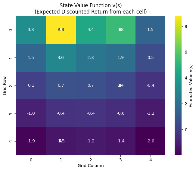
Explanation of Visuals
- The Heatmap: Represents . Lighter/brighter colors represent states with higher values.
- State A (0, 1): You will notice this cell has a high value. Even though moving out of A gives only , it transports you to , which might be in a safe area. The Bellman equation accounts for the immediate plus the value of being in .
- Edges: Cells near the edges often have lower values (darker colors) because the “random policy” bumps into walls frequently, incurring a reward of .