import numpy as np
import matplotlib.pyplot as plt

# --- 1. Environment Simulation ---
class UserEnvironment:
    def __init__(self):
        # Ads (Arms)
        self.ads = ["Tech_Gadget", "Retirement_Plan", "Fashion_Sale"]
        self.n_arms = len(self.ads)

        # Feature Mapping: [Bias, Age_Normalized, Is_Mobile]
        # Context dimension d = 3
        self.d = 3

    def get_user_context(self):
        """Simulate a random user visiting the site."""
        age = np.random.uniform(18, 70)
        is_mobile = np.random.choice([0, 1])

        # Normalize age to 0-1 range for stability
        age_norm = (age - 18) / (70 - 18)

        # Context vector: [Bias Term, Age, Device]
        context = np.array([1.0, age_norm, is_mobile])
        return context, age, is_mobile

    def get_reward(self, arm_index, context):
        """
        Simulate user clicking (Reward=1) or not (Reward=0) based on hidden preferences.
        Preferences (Unknown to algorithm):
        - Ad 0 (Tech): Likes Young people + Mobile users
        - Ad 1 (Retirement): Likes Older people + Desktop users
        - Ad 2 (Fashion): Random/General appeal
        """
        age_feature = context[1]  # 0.0 (young) to 1.0 (old)
        mobile_feature = context[2]

        # Calculate 'True' Probability of Click (CTR)
        if arm_index == 0: # Tech Gadget
            prob = 0.8 * (1 - age_feature) + 0.2 * mobile_feature
        elif arm_index == 1: # Retirement Plan
            prob = 0.8 * age_feature + 0.2 * (1 - mobile_feature)
        else: # Fashion
            prob = 0.15 # Low constant appeal

        prob = np.clip(prob, 0, 0.95) # Cap prob
return 1 if np.random.rand() < prob else 0This guide details the Contextual Upper Confidence Bound (LinUCB) algorithm.
In standard A/B testing or Multi-Armed Bandits (MAB), we treat all users the same. In Contextual Bandits, we assume the “best” ad depends on the user’s context (e.g., a 20-year-old on a mobile phone might prefer a Gaming Ad, while a 50-year-old on a Desktop might prefer an Investment Ad).
The algorithm balances Exploitation (showing the ad we think is best for this person) and Exploration (trying an ad we are uncertain about to learn more).
1. The Mathematical Model (LinUCB)
We use the Disjoint LinUCB algorithm. “Disjoint” means we learn a separate prediction model for each Ad (Arm).
For a specific Ad and a user with context vector (containing demographics/device data):
- Prediction: We predict the expected reward (Click-Through Rate) using a linear relationship:
where is the weight vector learned for Ad . 2. Confidence Interval (Uncertainty): We calculate how “unsure” we are about this prediction.
- is a matrix storing the covariance of contexts seen so far for Ad .
- is a hyperparameter controlling how much we want to explore.
- Decision Rule: Select the Ad that maximizes the Upper Confidence Bound:
2. Python Implementation & Visualization
This script simulates users with specific preferences, runs the LinUCB algorithm, and visualizes how it learns to target ads correctly over time.
# --- 2. LinUCB Algorithm ---
class LinUCB:
    def __init__(self, n_arms, n_features, alpha=2.5):
        self.n_arms = n_arms
        self.n_features = n_features
        self.alpha = alpha

        # Initialize A (Covariance) and b (Reward vector) for each arm
        # A is initialized as Identity matrix
        self.A = [np.identity(n_features) for _ in range(n_arms)]
        # b is initialized as zero vector
        self.b = [np.zeros(n_features) for _ in range(n_arms)]

    def select_arm(self, context):
        ucb_values = []

        for a in range(self.n_arms):
            # 1. Estimate Theta (Weight vector) -> theta = inv(A) * b
            A_inv = np.linalg.inv(self.A[a])
            theta = np.dot(A_inv, self.b[a])

            # 2. Predict Reward (Exploitation)
            pred_reward = np.dot(theta, context)

            # 3. Calculate Uncertainty (Exploration Bonus)
            # standard_deviation = sqrt(x.T * inv(A) * x)
            uncertainty = np.sqrt(np.dot(context.T, np.dot(A_inv, context)))

            # 4. Upper Confidence Bound
            ucb = pred_reward + self.alpha * uncertainty
            ucb_values.append(ucb)

        return np.argmax(ucb_values)

    def update(self, arm, context, reward):
        # Update A and b for the selected arm only
        # A += x * x.T
        self.A[arm] += np.outer(context, context)
        # b += reward * x
        self.b[arm] += reward * context
# --- 3. Simulation Loop ---
env = UserEnvironment()
agent = LinUCB(n_arms=env.n_arms, n_features=env.d, alpha=2.0)

n_rounds = 2000
ctr_history = []
clicks = 0
aligned_ad_choices = [] # To track if we showed 'correct' ad

for t in range(1, n_rounds + 1):
    # 1. A user arrives
    context, age_raw, is_mobile = env.get_user_context()

    # 2. Agent picks an Ad
    chosen_arm = agent.select_arm(context)

    # 3. User reacts (Click or No Click)
    reward = env.get_reward(chosen_arm, context)

    # 4. Agent learns
    agent.update(chosen_arm, context, reward)

    # Metrics
    clicks += reward
    ctr_history.append(clicks / t)

    # Heuristic check for visualization: Did we pick the "logic" best ad?
    # Young (<45) -> Tech(0), Old (>45) -> Retirement(1)
    if age_raw < 45 and chosen_arm == 0: aligned_ad_choices.append(1)
    elif age_raw >= 45 and chosen_arm == 1: aligned_ad_choices.append(1)
    else: aligned_ad_choices.append(0)
# --- 4. Visualizations ---
plt.figure(figsize=(12, 5))

# Plot 1: Click-Through Rate (CTR) Evolution
plt.subplot(1, 2, 1)
plt.plot(ctr_history, label="LinUCB CTR", color='blue')
plt.axhline(y=0.55, color='r', linestyle='--', label="Optimal CTR (approx)")
plt.xlabel("Rounds (Impressions)")
plt.ylabel("Cumulative CTR")
plt.title("Performance: Learning to Get Clicks")
plt.legend()
plt.grid(True)

# Plot 2: Decision Accuracy Moving Average
def moving_average(x, w):
    return np.convolve(x, np.ones(w), 'valid') / w

plt.subplot(1, 2, 2)
ma_window = 100
acc_ma = moving_average(aligned_ad_choices, ma_window)
plt.plot(acc_ma, color='green')
plt.xlabel("Rounds")
plt.ylabel(f"Alignment Accuracy (MA {ma_window})")
plt.title("Strategy: Learning User Segments")
plt.grid(True)
plt.ylim(0, 1)

plt.tight_layout()
plt.show()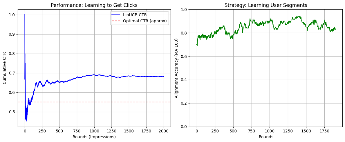
3. Deep Dive: What is happening in the code?
A. The Context Vector ()
In the get_user_context function, we turn a user into numbers.
- User: 25 years old, using an iPhone.
- Vector:
[1.0, 0.14, 1.0] 1.0: The bias term (essential for linear regression to find a baseline intercept).0.14: Normalized age (Young is close to 0, Old close to 1).1.0: Mobile device (Binary flag).
B. The Matrix (The “Memory”)
Each ad (arm) has its own matrix .
- Initially, is an Identity matrix. The algorithm knows nothing; the “uncertainty” term () is large for everyone.
- As we show Ad 0 to young people, the matrix changes shape. It “rotates” to align with the vector of young people.
- The math effectively asks: “Have I seen a vector like before for this ad?”
- Yes: The value is small Low Uncertainty Rely on prediction (Exploit).
- No: The value is large High Uncertainty Add huge bonus Pick this ad to learn (Explore).
C. The Alpha () Parameter
In LinUCB(..., alpha=2.0), this controls your risk appetite.
- High Alpha: The algorithm acts curious. It will show “Retirement Plans” to a 20-year-old just to be absolutely sure they don’t click on it.
- Low Alpha: The algorithm acts greedy. As soon as it sees one click from a young person on a “Tech” ad, it stops testing other ads and spams “Tech” to all young people.
4. Interpreting the Visualizations
If you run the code above, you will see two charts:
- Performance (Left Chart):
- The curve starts volatile (random guessing).
- It quickly stabilizes and trends upward.
- It should approach the “Optimal CTR” (red line). This proves the algorithm learned that showing random ads yields low clicks (~15%), but targeting yields high clicks (~50-60%).
- Strategy (Right Chart):
- This plots “Alignment Accuracy.” It asks: Did the algorithm show the Tech Ad to a young person or the Retirement Ad to an older person?
- Initially, this will hover around 0.33 (random chance among 3 ads).
- Over time, it will rise toward 0.9 or 1.0, showing that the algorithm has successfully “segmented” the users without us explicitly programming
if age < 30.